The task of circle fit is a very popular one and it often makes its appearance in machine vision applications. Also the problem of solving a task in a least squares sense comes out repeatedly. As it turns out the former could be used to nicely illustrate snags of the latter. Today I would like to discuss what does it mean to fit a circle in a least square sense and if it leads to an unambiguous solution. I will base my example on two rather old but very informative papers:

Gander W. Golub G.H. Strebel R. Least–Squares Fitting of Circles and Ellipses BIT Numerical Mathematics, 34(4) pp. 558–578, 1994
Coope L.D. Circle fitting by linear and nonlinear least squares Journal of Optimization Theory and Applications, 76(2) pp. 381–388, 1993

First, lets define the problem at hand. The task is to find a radius and center of a circle best fitting a set of points on the plane. The points may not necessarily lie perfectly on a circumference of a circle, may not be evenly distributed and their number may vary, however it is always greater than the number of sought for parameters.

The algebraic approach

The most straightforward approach is to consider an algebraic representation of a circle on a plane:

$F(\boldsymbol{x}) = a\boldsymbol{x}^T\boldsymbol{x} + \boldsymbol{b}^T\boldsymbol{x} + c = 0$

where:

$\boldsymbol{x}^T = \left[\begin{array}{cc}x & y\end{array}\right]$

Having m data points we can build an overdetermined set of linear equations

$B\boldsymbol{u} = 0$

for unknown coefficients

$\boldsymbol{u} = \left[\begin{array}{cccc}a & b_x & b_y & c\end{array}\right]^T$

, where:

$B = \left[\begin{array}{cccc} x_{1}^2 + y_{1}^2 & x_{1} & y_{1} & 1 \\ \vdots & \vdots & \vdots & \vdots \\ x_{m}^2 + y_{m}^2 & x_{m} & y_{m} & 1 \end{array}\right]$

If the number of points

$m > 3$

the system most likely does not have a solution, unless all points actually lie on the circle. Therefore, in order to get a result, it is required to impose an additional constraint, such as

$||\boldsymbol{u}|| = 1$

. We obtain a total least squares problem:

$||B\boldsymbol{u}|| = \min$

s.t.

$||\boldsymbol{u}|| = 1$

According to the 1st referenced paper the solution can be found from the right singular vector of matrix

$B$

associated with the smallest singular value. More insight on the TLS problem can be found in this paper. In order to extract the center and radius of the circle the algebraic equation should be transformed to the form as below:

$\left(x + \frac{b_x}{2a}\right)^2 + \left(y + \frac{b_y}{2a}\right)^2 = \frac{||\boldsymbol{b}||^2}{4a^2} - \frac{c}{a}$

Now the circle parameters are easily defined as:

$(x_{c}, y_{c}) = \left(-\frac{b_x}{2a}, -\frac{b_y}{2a}\right) \\ r = \sqrt{\frac{||\boldsymbol{b}||^2}{4a^2} - \frac{c}{a}}$

To see how this approach works in practice we can easily code it in Matlab. For this test, as well as for upcoming ones, we are going to use a small data set as defined in the referenced paper.

$P = \left[\begin{array}{cccccc} 1 & 2 & 5 & 7 & 9 & 3 \\ 7 & 6 & 8 & 7 & 5 & 7 \end{array}\right]^T$

P = [1 7; 2 6; 5 8; 7 7; 9 5; 3 7];
B = [(P.*P)*[1 1]‘, P(:,1), P(:,2), ones(6, 1)];
[U,S,V] = svd(B);
d = diag(S);
res = V(:, find(d == min(d)));
xc = –res(2)/(2*res(1));
yc = –res(3)/(2*res(1));
r = sqrt((res(2)^2 + res(3)^2)/(4*res(1)^2) – res(4)/res(1));

The script builds the

$B$

matrix, calculates its SVD decomposition and chooses eigenvector corresponding to the smallest eigenvalue. Finally, it transforms the solution of the linear system to the desired circle parameters. The resulting circle is plotted in the figure below.

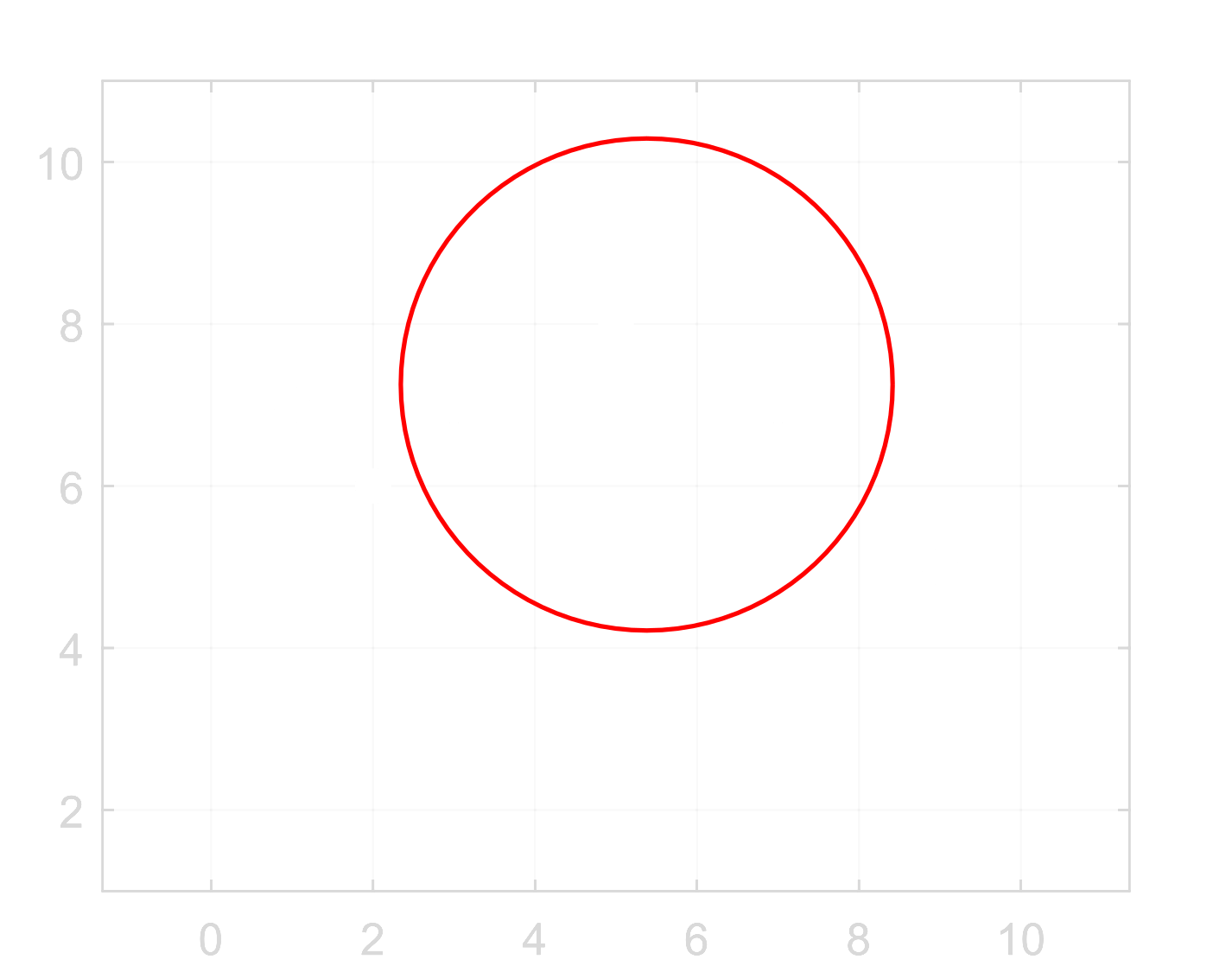
Now, the question arises if this is the desired outcome and why we have got a result other than expected? It turns out that the algebraic approach yields a circle lying the closest to the input set of points but does not take into account its geometric relationships. Therefore the result is most likely not satisfactory, especially if the number of sampled points is small or they are not evenly distributed. Is there another way to fit a circle in a more reasonable way?

The geometric approach

The problem with the algebraic approach was that we really didn’t realize what we were actually minimizing. Now we will try to define the cost function, so that it minimizes sum of squares of distances between the desired radius and a sector between the center and each sampled point, as indicated in the picture.

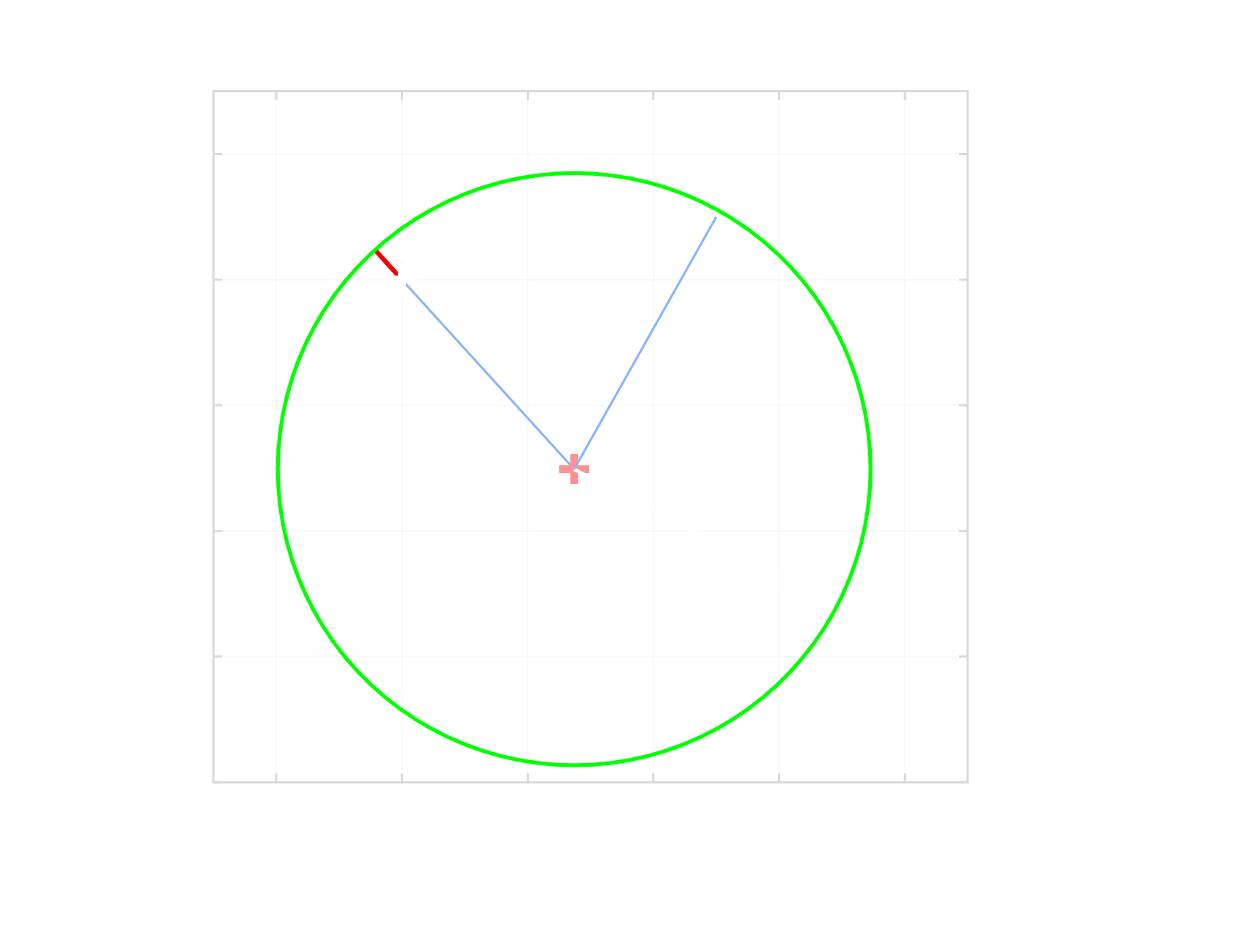
This residual for a data point

$\boldsymbol{x}_i = [x_i, y_i]$

and circle center

$\boldsymbol{c} = [x_c, y_c]$

can be written as:

$d_i^2 = \left(||\boldsymbol{c} - \boldsymbol{x}_i|| - r\right)^2$

or after expansion:

$d_i^2 = \left(\sqrt{(x_{c} - x_{i})^2 + (y_{c} - y_{i})^2} - r\right)^2$

Thus, the cost function to minimize is the sum of residuals for all data points:

$f(x_{c}, y_{c}, r) = \sum_{i=1}^m d_i(x_{c}, y_{c}, r)^2$

This time the task is described well in the geometric sense but we face a different difficulty. The resulting least squares problem is a non-linear one, so that there is no a straightforward analytical solution. Instead we have to use an iterative approach. In this case we can take advantage of the Gauss-Newton algorithm and, simultaneously, explain this approach in more details.

Gauss-Newton algorithm

The algorithm is a modification of the Newton’s method in optimization which minimizes a sum of squares, just like the one we came upon in the circle fit problem. One advantage over the Newton’s method is that it does not require to calculate partial second derivatives of the objective function (the Hessian). Just the first derivatives (the Jacobian) is sufficient.

In data fitting problem the components of the minimized sum are the residuals which are differences between data points and values predicted by a model. In our case these are precisely the squared differences that we defined above. They describe deviations between the modeled radius of a fitted circle and actual distance between a data point an the circle center.

The Gauss-Newton algorithm approximates the solution step by step by updating the sought for model parameters in each iteration according to the procedure:

$f^{(n+1)} = f^{(n)} - J_r^*\boldsymbol{d}\left(f^{(n)}\right)$

where

$J_r^*$

is the inverse of the Jacobian of residuals and

$\boldsymbol{d}$

are the residuals.

In case of an overestimated system, where there are more data points than model parameters, the Jacobian matrix is rectangular and thus non-invertible. Therefore a pseudoinverse is used instead:

$J_r^* = \left(J_r^T J_r\right)^{-1}J_r^T$

In order to find the Jacobian we need to calculate partial derivatives with respect to all model parameters (

$x_c, y_c, r$

) and evaluate them for each data point:

$J(x_{c}, y_{c}, r) = \left( \begin{array}{ccc} \frac{\delta d_1(x_{c}, y_{c}, r)}{\delta x_{c}} & \frac{\delta d_1(x_{c}, y_{c}, r)}{\delta y_{c}} & \frac{\delta d_1(x_{c}, y_{c}, r)}{\delta r} \\ \vdots & \vdots & \vdots \\ \frac{\delta d_m(x_{c}, y_{c}, r)}{\delta x_{c}} & \frac{\delta d_m(x_{c}, y_{c}, r)}{\delta y_{c}} & \frac{\delta d_m(x_{c}, y_{c}, r)}{\delta r} \end{array} \right)$

Which in case of our residuals

$d_i$

will be:

$J(x_{c}, y_{c}, r) = \left[ \begin{array}{ccc} \frac{x_{c} - x_{1}}{\sqrt{(x_{c} - x_{1})^2 + (y_{c} - y_{1})^2}} & \frac{y_{c} - y_{1}}{\sqrt{(x_{c} - x_{1})^2 + (y_{c} - y_{1})^2}} & -1 \\ \vdots & \vdots & \vdots \\ \frac{x_{c} - x_{m}}{\sqrt{(x_{c} - x_{m})^2 + (y_{c} - y_{m})^2}} & \frac{y_{c} - y_{m}}{\sqrt{(x_{c} - x_{m})^2 + (y_{c} - y_{m})^2}} & -1 \end{array} \right)$

Now we are ready to implement and test this solution.

Implementation

To start calculations we have to define initial values for the center and radius of the circle. For this purpose we can use results of the algebraic fit from the first example and store them as a vector.

xc = 5.3794;
yc = 7.2532;
r = 3.0370;
res = [xc; yc; r];

The iterative procedure of Gauss-Newton algorithm can be implemented as follows:

max_iters = 20;
max_dif = 10^(-6); % max difference between consecutive results
for i = 1 : max_iters
    J = Jacobian(res(1), res(2), P);
    R = Residual(res(1), res(2), res(3), P);
    prev = res;
    res = res - J\R;
    dif = abs((prev - res)./res); 
    if dif < max_dif
        fprintf('Convergence met after %d iterations\n', i);
        break;
    end
end
if i == max_iters
    fprintf('Convergence not reached after %d iterations\n', i);
end

First we define two exit conditions, either if the result between two consecutive iteration barely changes or if the maximum number of iteration has been reached before convergence. Next, we use helper functions to calculate the Jacobian and the residuals vector. After that, we find the new approximation of the result and check the exit conditions.

The Jacobian and Residual helper functions are implemented below:

function J = Jacobian(xc, yc, P) 
    s = size(P);
    denom = sqrt((xc - P(:,1)).^2 + (yc - P(:,2)).^2);
    J = [(xc - P(:,1))./denom, (yc - P(:,2))./denom, -ones(s(1), 1)];
end

function R = Residual(xc, yc, r, P)
    R = sqrt((xc - P(:,1)).^2 + (yc - P(:,2)).^2) - r;
end

The final result reached after 11 iterations is shown in the following figure.

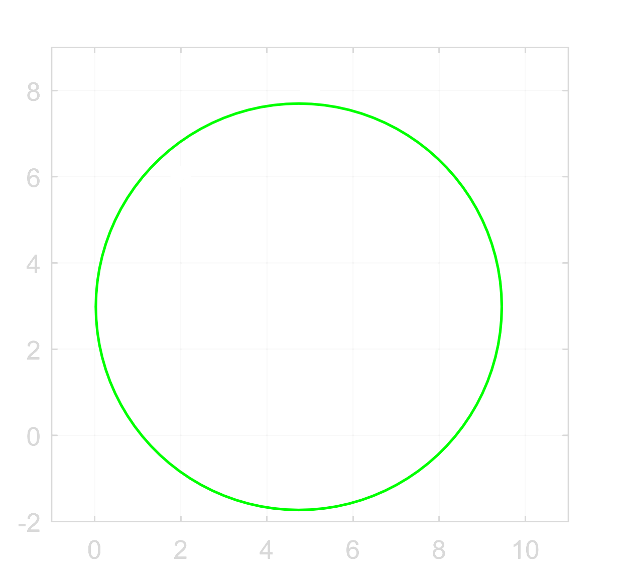
This time the outcome is in line with the common sense because the data points are located along an arc of a circle. This result however does not come without an extra cost. The disadvantage of a non-linear least squares optimization is the fact that it guarantees to find a local minimum only. Therefore the final result depends on the choice of a starting point and a poor shot can lead to a lack of convergence at all. Let’s see if there is anything that we can do about it.

Linearized geometric approach

Previously we defined the squares of residuals as

$d_i^2 = \left(||\boldsymbol{c} - \boldsymbol{x}_i|| - r\right)^2$

which resulted in a non-linear optimization problem. We can however modify their definition slightly, having in mind that we commit some estimation error and in consequence solve a little bit different problem. Consider the residuals defined as follows:

$g_i = \left(||\boldsymbol{c} - \boldsymbol{x}_i||\right)^2 - r^2$

After expansion of the first term and rearrangement we get:

$g_i(\boldsymbol{c}, r) = \boldsymbol{x}_i^T \boldsymbol{x}_i - 2\boldsymbol{c}^T \boldsymbol{x}_i - \left(r^2 - \boldsymbol{c}^T \boldsymbol{c}\right)$

Now, remembering that we seek for the center of a circle c and its radius r, we can rearrange the equation further:

$g_i(\boldsymbol{c}, r) = \boldsymbol{x}_i^T \boldsymbol{x}_i - \left(2\boldsymbol{c}^T \boldsymbol{x}_i + \left(r^2 - \boldsymbol{c}^T \boldsymbol{c}\right)\right)$

$g_i(\boldsymbol{c}, r) = \boldsymbol{x}_i^T \boldsymbol{x}_i - \left[\begin{array}{cc}\boldsymbol{x}_i^T & 1 \end{array}\right] \left[\begin{array}{c}2\boldsymbol{c}\\ r^2 - \boldsymbol{c}^T \boldsymbol{c}\end{array}\right]$

And make a clever substitution of variables:

$\boldsymbol{z} = \left[\begin{array}{c}2x_c\\ 2y_c\\ r^2 - \boldsymbol{c}^T \boldsymbol{c}\end{array}\right]$

Finally, we get the residual defined as:

$g_i(\boldsymbol{c}, r) = \boldsymbol{x}_i^T \boldsymbol{x}_i - \left[\begin{array}{cc}\boldsymbol{x}_i^T & 1 \end{array}\right]\boldsymbol{z}$

which is linear with respect to the variable z. Now, the sum of squares of the residuals

$g_i(\boldsymbol{c}, r)$

becomes a linear least squares problem:

$\min_{\boldsymbol{z}}\sum_{i=1}^m \left(\boldsymbol{x}_i^T \boldsymbol{x}_i - \left[\begin{array}{cc}\boldsymbol{x}_i^T & 1 \end{array}\right]\boldsymbol{z}\right)^2$

which is equivalent to solving a linear system

$B\boldsymbol{z} = \boldsymbol{y}$

, where

$B$

incorporates vectors

$\left[\begin{array}{cc}\boldsymbol{x}_i^T & 1 \end{array}\right]$

and

$\boldsymbol{y}$

is equivalent to a vector of products

$\boldsymbol{x}_i^T \boldsymbol{x}_i$

for all data points.

It has a unique solution if at least 3 columns in the matrix

$B$

are linearly independent. The solution can be found from normal equations and becomes:

$\boldsymbol{z} = \left(B^TB\right)^{-1}B^T\boldsymbol{y}$

One final step is to restore the original variables, so that:

$x_{c} = \frac{1}{2}z_1$

$y_{c} = \frac{1}{2}z_2$

$r = \sqrt{z_3 + \boldsymbol{c}^T\boldsymbol{c}}$

Now is the time to see how the linearized geometric approach works in practice. Here is the Matlab code:

[n, m] = size(P);
y = [P, ones(n, 1)]\sum(P.*P, 2);
x = 0.5*y(1:m);
r = sqrt(y(m+1) + x'*x);

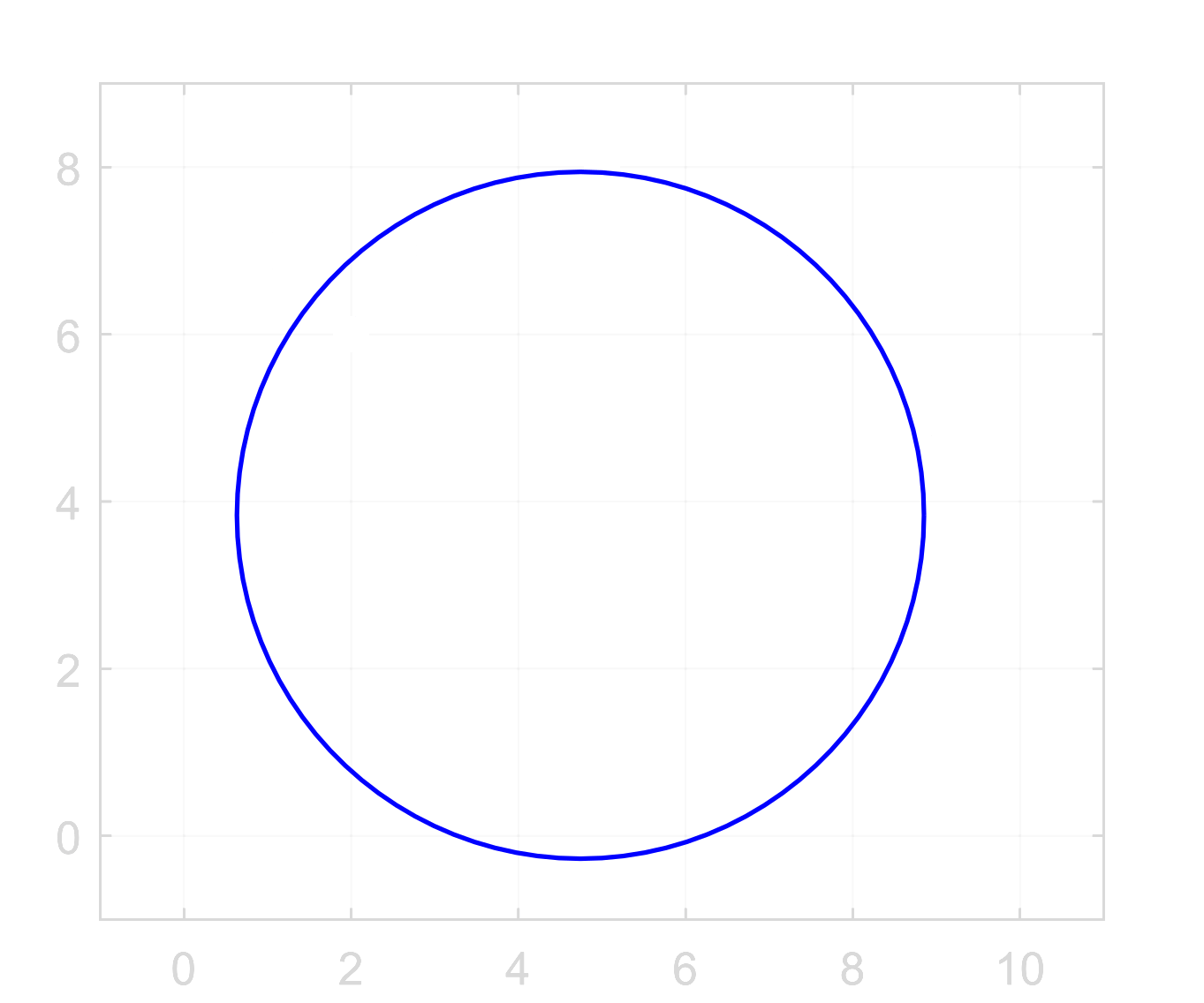
Below you can see the plot of the fitted circle:

Conclusions

We discussed three different approaches to least squares circle fit. Each of them presents its own advantages and shortcomings. Their combined results are shown in the figure below. It is clearly visible that they may differ greatly. In a real world scenario however, the number of data points would be significantly larger which would most likely diminish the scale of differences. Nevertheless it is worth knowing they persist.

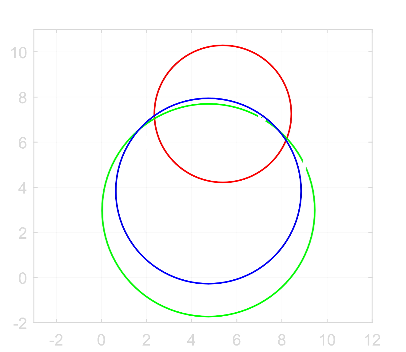
The algebraic method provides a simple solution, yet it does not define the cost function in a geometric context, therefore its result could be unexpected. Usually it provides the first approximation for an iterative algorithm.

The geometric approach formulates the problem correctly in the geometric sense but yields a non-linear least squares problem which is much harder to solve. It requires an iterative solver which is numerically expensive, affected by a choice of a starting point and does not guarantee to converge. However, once the initial conditions are well defined it provides the most expected solution.

The linearized approach overcomes the shortcomings of the geometric one at the cost of skewing the result by changing the cost function.

A conclusion to remember is that a fit in a least squares sense is a family of optimization methods which take different approach in formulating the problem at hand and use different mathematical means to solve it. It is always important to realize what task do we want to solve and select the right tool to do it.